 Vladimir V. Kostromin
Political scientist, vkostromin@eu.spb.ru
Vote Use under Multiple Nontransferable Vote: An Aggregate Analysis of Russian Municipal Elections
Abstract
The multiple nontransferable vote system (MNTV) gives voters several votes, which they may use at their discretion. The number of votes actually cast by voters appears to be an important indicator of how this electoral system functions. In most previous studies, however, this measure has been used only as an auxiliary indicator, with little attempt to explain what may account for its variation. This study seeks to conceptualize the number of votes used by voters as a reflection of the relationship between existing electoral demand and the supply offered by parties and candidates. This conceptual framework suggests that voters' failure to use some of the votes available to them may be associated with insufficient satisfaction of electoral demand. Accordingly, the emergence of the necessary supply should be associated with the use of a larger number of votes. Building on this approach, the study formulates empirically testable hypotheses that explain the conditions under which voters make more or less active use of the votes available to them. In this article, electoral demand is examined with reference to possible criteria that voters use when selecting candidates, derived from voting methods. These assumptions are tested on a large dataset of Russian municipal elections, covering cities of the Russian Federation as well as intra-city municipal formations in Moscow and St. Petersburg from 2007 to 2021. The results show that vote use by Russian voters is more consistent with a "free-choice" voting model, which assumes that voters select candidates based on their individual characteristics. By contrast, the "party-based" voting model, which implies support only for candidates nominated by the voter’s preferred party, receives weak empirical support.
Introduction
The multiple non-transferable vote system (MNTV [11: 14–15]) gives voters several votes. They may use these votes at their discretion: cast the minimum number, use only some, or all of them [21: 44]. This feature gives the voters flexible opportunities to express their preferences. Although the intensity with which voters use their votes appears to be an important aspect of the MNTV electoral system [15: 472], most studies use this indicator only as a descriptive measure or limit themselves to testing possible correlations [10: 930; 15: 472–474; 16; 17; 20: 115–116]. Only a small number of studies examine the conditions associated with voters’ use of a larger or smaller number of votes [19].
This study attempts to propose a conceptual framework that treats the number of votes used by voters as the result of an interaction between emerging electoral demand and the existing supply provided by parties and candidates. It is assumed that voters are willing to use the votes available to them when demand is satisfied by supply, and vice versa. This approach involves identifying the factors of electoral supply that are most strongly associated with vote use. The results obtained make it possible to infer which type of electoral demand is more widespread among voters.
Electoral demand is understood here as the principle by which suitable candidates are selected. Approaches to such selection can be described through the voting models preferred by voters under MNTV. Thus, the "party-based" voting model assumes that a voter votes only for candidates from the preferred party. In this case, using all votes is possible if the supported party has full representation in the constituency. The "free-choice" voting model involves voters selecting candidates based on their own preferences. Using all available votes is possible if the voter finds candidates who correspond to their views. Finding evidence in favor of particular types of electoral demand makes it possible to infer the likely consequences of using the MNTV system.
However, this type of analysis is most often complicated by the absence of data on individual vote use. This study proposes using the average share of additional votes used by voters as the most convenient and appropriate aggregate measure of the number of votes used. The advantage of this approach is that it provides a unified scale range regardless of the magnitude of the constituency under analysis.
The search for relationships between factors of electoral supply and the aggregate measure of the number of votes used is conducted using data from Russian municipal elections held under the MNTV system. Previous studies have noted that Russian voters make relatively infrequent use of the voting potential available to them [10: 930; 15: 472–474; 16; 17]. This study seeks to demonstrate which factors of electoral supply are more strongly associated with more intensive vote use.
The analysis described is conducted on a large dataset of municipal elections in Russia. It covers three electoral cycles from 2007 to 2021 and includes elections in various municipal formations across Russian regions. The analytical strategy is based on the use of a mixed multilevel regression model, which makes it possible to account for the hierarchical structure of the data. The results obtained are more consistent with the assumption that Russian voters more often use the "free-choice" rather than the "party-based" voting model.
Vote Use under the Multiple Non-Transferable Vote System
Multiple Non-Transferable Vote system (MNTV) [11: 14–15], is an electoral system in which voters have several votes at once. The number of votes is equal to the number of seats to be filled in the constituency (\(V = M\)) [21: 44]. Voters cast their votes for individual candidates and may choose representatives of different parties at the same time. However, each candidate may be supported only once; that is, cumulative voting is not permitted. The seats are won by the \(M\) candidates who receive a relative majority of votes in the constituency.
This combination of electoral rules gives voters a wide range of voting opportunities [6; 12; 20]. The availability of several votes, together with the possibility of choosing representatives of different parties, allows voters to form combinations of candidates that best reflect their preferences. In addition, the possibility of using only some of the available votes [21: 44] further expands voters' choices. This possibility allows voters to support only the most suitable candidates and avoid contributing to the victory of those who, for one reason or another, do not meet their preferences.
The number of votes used by voters appears to be an important indicator of how the MNTV system functions [15: 472–474]. Its value may indicate the degree of correspondence between voters' electoral demand and the supply provided by parties or candidates. If a large share of voters does not use the votes available to them, this may serve as evidence of a gap between the candidates the voters need and those available [19: 5]. Voters' demand may be variable and heterogeneous. However, it can be examined in terms of possible approaches to voting under MNTV, which makes it possible to distinguish different types of electoral demand.
Voting models under MNTV are ideal types that describe approaches to voting based on voters' selection of candidates. For example, voters may view an election either as a contest between parties or as a competition among individual candidates [6: 266–268]. Each of these approaches produces a distinct model for selecting fitting candidates. In the first case, which may be described as the "party-based" model, choice is limited to representatives of the preferred party. In the second case, which may be described as the "free-choice" model, voters consider all candidates and select the most suitable ones according to their own preferences. The consequences of using the MNTV system may depend on the voting model that is most widespread among voters [12: 104–105]. This makes the prevailing voting model an important element in the functioning of this electoral system.
Electoral demand of voters is shaped by the voting model they use. This is because each model defines in its own way which of the available candidates are fitting. However, regardless of the model used and the demand it generates, the mechanism of vote use remains the same: voters use the votes available to them if there are fitting candidates. More formally, this means that their electoral demand is matched by a corresponding supply. Conversely, if supply is smaller than demand, voters can use only some of the votes available to them. Since each model produces its own version of demand, it is necessary to examine in more detail the basis on which this demand is formed.
Under the "party-based" voting model, voters are assumed to rely mainly on party labels when deciding how to vote [22: 560–561]. In this case, a voter supports the preferred party by voting for each of its nominated candidates and ignoring all other candidates running in the election. This voting model implies that the voter has demand only for representatives of the party they support. Supply, in this case, is the number of such candidates in the election. This means that a voter who relies on the "party-based" model uses all available votes if each available vote corresponds to a candidate from the supported party. Conversely, if the available supply is insufficient, that is, if the number of required candidates is smaller than the number of votes available, only some of the votes are used because demand is not fully satisfied.
Under the "free-choice" voting model, voters are assumed to consider all candidates available to them without limiting themselves to any single party [20: 113]. To make an informed choice among them, a voter uses their preferences to identify certain important candidate characteristics. The voter then uses these criteria to select the most fitting candidates and votes for them.
This approach implies that each voter's demand is individualized and depends on their own preferences. This demand is expressed in the form of candidates fitting certain required criteria. Such criteria may include socio-demographic characteristics that are important to the voter, ideological position, views on specific policy issues, etc. Accordingly, the demand of a particular voter will be satisfied if the election includes the required number of candidates who meet the criteria selected by that voter. As a result, supply is the number of candidates who meet the specified conditions. In this case, the more candidates correspond to the criteria formed by the voter, the larger the number of votes that will be used, and vice versa.
Conceptualizing the use of available votes under MNTV as an interaction between electoral demand and supply makes it possible to identify the conditions under which a larger or smaller number of votes is used. This approach suggests that, for a voter to use each additional vote, there must be an additional candidate who corresponds to the relevant demand. A voter can use all available votes when existing electoral demand and supply correspond to each other. If this correspondence is achieved only partially, only some of the votes are used. In the most extreme case, if electoral demand is not satisfied at all, the voter may abstain from voting.
This approach to analyzing vote use proceeds from the assumption that voters are interested in using all available votes. This means that each vote has equal value and that casting each of them is equally beneficial. In this case, the use of each subsequent vote depends only on whether there is an opportunity to do so. The initial assumption also implies that voters who are not willing to use all available votes follow a different mechanism of vote use. Their participation in the election should not interfere with the analysis, since they are guided by different incentives.
Thus, the number of votes used by voters under MNTV may be an important indicator reflecting the difference between the demand formed by voters and the supply available in the election from parties and candidates. A large number of unused votes may provide evidence of a substantial gap between these structural factors, and vice versa. In addition, identifying stable and substantial relationships between different factors of electoral supply and the potential for vote use may provide evidence in favor of particular voting models, thereby contributing to a better understanding of how MNTV functions.
Estimating the Number of Votes Used
A direct estimate of the number of votes used requires data on the voting behavior of each participating voter. In most cases, however, such information is unavailable. Election results are most often presented as aggregate results for parties or candidates within a particular territory, such as a polling station (precinct), constituency, etc. This limitation makes it possible to calculate the number of votes used by voters only in aggregate form.
This estimate represents the average number of votes used by voters within a given territory. For convenience, the discussion below assumes that it is calculated at the level of the polling station (\(i\)). To calculate it, it is necessary to use data on the total number of votes cast by voters (\(VT\) – Voters Total), which can be calculated as the sum of all votes received by the candidates. It is also necessary to know the number of voters whose ballots are valid (\(VB\) – Valid Ballots). The ratio of these two values is defined as the average number of votes used by voters (\(AUV\) – Average Used Votes):
$$AUV_{id} = \frac{VT_{id}}{VB_{id}}=\frac{\sum_{1}^{N_{d}}v_{cid}}{VB_{id}}\quad(1) ,$$
where \(i\) is the number of the polling station, \(d\) is the number of the electoral district, \(N_d\) is the number of candidates in district \(d\), \(c\) is the identifier of a candidate running in the election, and \(V_{cid}\) is the number of votes received by candidate \(c\) at polling station \(i\) in constituency \(d\).
The average number of votes used (\(AUV_{id}\)) is an aggregate value that reflects how many votes voters used on average at a given polling station. The possible range of this variable is determined by the constituency size and extends from 1 to \(M\). Thus, the closer the resulting value is to 1, the fewer votes were used on average by one voter. The closer this value is to \(M\), the greater the number of votes used on average.
The average number of votes used by voters does not necessarily correspond to the most frequent pattern of vote use among voters at a given polling station. Since this measure is an aggregate value, there may be cases in which the number of votes most commonly used by voters at a particular polling station differs substantially from the mean value. Therefore, this indicator should be interpreted as a value reflecting how fully voters use the votes available to them on average.
A drawback of this approach to estimating the aggregate number of votes used is that the scale depends on constituency size. This feature is critical when studying constituencies of different sizes. It is therefore useful to construct an alternative measure with a unified range. To do this, min-max normalization should be applied.
This procedure requires adjusting the numerator and the denominator of the average number of votes used (\(AUV\)). The minimum possible number of votes that could have been cast by voters must be subtracted from the numerator. This value is equal to the number of valid ballots (\(VB\)). The denominator, in turn, must be multiplied by the maximum possible number of additional votes. This value is expressed as constituency size minus one (\(M - 1\)). Thus, the numerator contains the total number of additional votes cast by voters (\(AVT\) – Additional Votes Total), while the denominator contains the maximum possible number of additional votes available to voters (\(AVP\) – Additional Votes Potential). In this case, the final formula is as follows:
$$ASUAV_{id} = \frac{AVT_{id}}{AVP_{id}} = \frac{VT_{id} - VB_{id}}{VB_{id} \times (M_{d} - 1)}\quad(2) ,$$
This transformation creates a unified scale, where 0 corresponds to the use of one vote and 1 corresponds to the use of \(M\) votes. In this case, the variable is best understood as the average share of used additional votes (\(ASUAV\) – Average share of used additional votes). It reflects what share of additional votes was used by voters on average. The closer the value is to 1, the larger the share of additional votes used by voters on average, and vice versa. In other words, this measure captures the intensity with which voters use the additional votes available to them.
This interpretation of the indicator follows from a change in the starting point of measurement. Since this indicator covers only valid ballots, the use of at least one vote is a necessary condition. The remaining available votes (2, M) can be regarded as additional. Focusing on these votes is of greatest interest because the extent to which they are used depends directly on the correspondence between electoral demand and supply.
The relationship between the average number of votes used (\(AUV\)) and the average share of used additional votes (\(ASUAV\)) can be seen in Figure 1: across different constituency sizes, the relationship remains linear, with only the slope varying. This makes it possible to convert values from one measure into the other:
$$AUV_{id} = ASUAV_{id} \times (M_{d} - 1) + 1\quad(3)$$
$$ASUAV_{id} = \frac{AUV_{id} - 1}{(M_{d} - 1)}\quad(4) $$
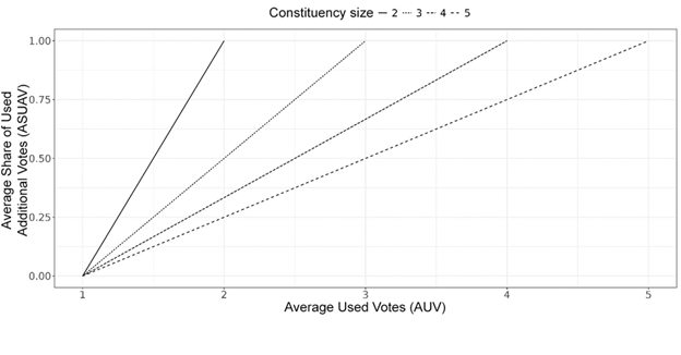
Figure 1. Comparison of Different Approaches to Estimating the Aggregate Number of Votes Used
The few existing studies of the number of votes used under MNTV have employed a different approach to calculating the aggregate measure [15: 472; 19: 4–5]. Under this approach, the minimum value of the scale depends on constituency size, which may create difficulties for analysis. Therefore, the proposed aggregate measure based on the average share of used additional votes appears more practical, since it has a unified range.
Vote Use in Russian Municipal Elections
The number of votes used under MNTV has received only limited attention in previous studies [8: 486–487; 10: 930; 15: 472–474; 16; 17; 19; 20: 115–116]. However, as shown above, this indicator is an important component of the electoral system. Accordingly, identifying the conditions associated with more or less intensive vote use makes it possible to gain a deeper understanding of how the MNTV system functions.
This study focuses on the case of Russian municipal elections held under the MNTV system. Previous studies have noted that, in the Russian context, this electoral system does not produce the expected consequences [10]. The "sweep effect," which implies one party winning all seats in a constituency [25: 193], has occurred much less frequently in Russian elections [10; 15: 138–139]. This feature has been explained by the fact that voters do not use the full voting potential available to them [10: 429–430; 15: 138–139], a pattern confirmed by aggregate data [10: 430; 15: 472–474; 16; 17].
The voting models used by Russian voters may offer an additional explanation for the limited occurrence of the "sweep effect." The "free-choice" voting model limits the conditions under which this effect can arise, because in this case voters select candidates according to different criteria rather than party affiliation alone. If voters tend to prefer the "party-based" model, which facilitates the "sweep effect," it becomes necessary to identify additional factors that prevent this effect from occurring more often.
It should be noted that the proposed mechanisms of interaction between electoral demand and supply have so far been described at the individual level. At the aggregate level, this approach remains relevant if the interaction described above is structural in nature. In that case, an increase in the number of voters who refrain from using some of their votes at the individual level should lead to a decrease in the aggregate measure of vote use, and vice versa. On this basis, we formulate empirically testable hypotheses about how the previously introduced average share of used additional votes is related to electoral supply factors associated with each voting model.
If some Russian voters follow the "party-based" voting model, then, all else being equal, the absence of some candidates from their preferred party should reduce the number of votes used by that party’s supporters. The hypothesis can be formulated as follows:
H1: The average share of used additional votes is negatively associated with a party’s incomplete candidate representation in an electoral constituency.
This hypothesis is formulated in general terms and requires specification for individual parties in the form of additional hypotheses. The relevant cases are parties that take active part in elections and potentially have a large number of supporters. The main parliamentary parties – United Russia, CPRF, LDPR, A Just Russia – meet these conditions. If the expected relationship exists, it should primarily concern these parties. It also seems relevant to include Yabloko, which conducted active electoral campaigns in the municipalities of Moscow and St. Petersburg. For each of these parties, we formulate an additional hypothesis:
H1a: The average share of used additional votes is negatively associated with United Russia being represented in an electoral constituency by an incomplete number of candidates;
H1b: The average share of used additional votes is negatively associated with CPRF being represented in an electoral constituency by an incomplete number of candidates;
H1c: The average share of used additional votes is negatively associated with LDPR being represented in an electoral constituency by an incomplete number of candidates;
H1d: The average share of used additional votes is negatively associated with A Just Russia being represented in an electoral constituency by an incomplete number of candidates;
H1e: The average share of used additional votes is negatively associated with Yabloko being represented in an electoral constituency by an incomplete number of candidates.
If the voting behavior of some Russian voters corresponds to the "free-choice" model, the number of votes used should decrease when candidates with the required characteristics are absent. However, it is difficult to identify a single variable that would capture the extent to which electoral demand is satisfied for all voters at once, since voters differ in the criteria they use to select candidates. Nevertheless, it is possible to identify a variable that affects the likelihood that each voter's demand will be satisfied. Candidate diversity appears to be such a measure. The more varied the candidates running in an election are, the more likely voters with different selection criteria are to find suitable candidates, and vice versa. The hypothesis can therefore be formulated as follows:
H2: The average share of used additional votes is positively associated with candidate diversity in an electoral constituency.
Here, candidate diversity refers to differences among candidates. It can be measured in two ways. The first approach uses the number of candidates in a constituency as a proxy for diversity. It is reasonable to expect a positive monotonic relationship between the number of candidates and the level of diversity: the more candidates compete in the constituency, the higher the expected level of diversity.
The second approach constructs a partial measure of diversity based on the number of unique candidate profiles, defined by candidates' socio-demographic characteristics. This information is available to voters when they cast their ballots. However, it is unclear to what extent voters rely on it when selecting candidates, or whether they also use any additional information about them. For this reason, the proposed measure captures only a limited aspect of existing diversity: on average, the more candidates with unique profiles there are, the higher the level of diversity in the constituency, and vice versa.
Neither of the two proposed approaches provides an ideal way to measure the diversity in a constituency. However, both can be expected to correlate with it. Using several measures at the same time makes the results more reliable. The hypothesis formulated above can therefore be specified through the following additional hypotheses:
H2a: The average share of used additional votes is positively associated with the number of candidates in the constituency;
H2b: The average share of used additional votes is positively associated with the number of unique profiles in the constituency.
As a result, the hypotheses are designed to test whether the aggregate measure of vote use is associated with electoral supply factors relevant to different voting models. The "party-based" model is examined through the H1 hypotheses, while the "free-choice" model is examined through the H2 hypotheses. If the relationships identified are stable and substantial, they will provide indirect evidence of the use of different voting models in the context of Russia.
Data
To test the hypotheses, the study uses several datasets covering municipal elections held under the MNTV system in Russia from late 2007 to late 2021. This electoral system is actively used in elections to intracity municipal formations (IMFs) of Moscow and intracity municipal formations of St. Petersburg. It is also fairly widespread in municipalities of various levels across Russian regions.
At present, however, covering all municipalities in Russian regions is problematic. For this reason, the analysis focuses on selected cities. This choice is justified, on the one hand, by the fact that cities are compact territorial units where voter density is high. On the other hand, the number of cities is limited and sufficient for the purposes of the analysis. During the period under study, in terms of municipal structure, cities could be either urban okrugs (first-level MFs) or urban settlements (second-level MFs). For this reason, we will further refer to them as urban municipal formations (UMFs).
For UMFs, the sample included only cases in which the city had its own representative body. If a municipality was reorganized (e. g., incorporated into another municipality or transformed into a different type of okrug) and no longer had a representative body relevant to the city, the larger unit was excluded from the sample. Earlier cases remained in the sample. For IMFs, the number of included cases corresponds to the official territorial structure at the time of the elections. This means, for example, that the municipalities of New Moscow are included in the analysis only from the moment of their incorporation into Moscow.
This sample covered 1,034 UMFs, 146 IMFs of Moscow, and 111 IMFs of St. Petersburg. It included all available regular elections from late 2007 to late 2021, covering three full electoral cycles. All information on electoral statistics and candidates’ socio-demographic characteristics was obtained from the official website of the Central Election Commission of the Russian Federation (the CEC or Russia), and the State Automated System "Elections" (SAS Vybory).
For the purposes of this analysis, only those municipalities in the previously described sample where elections were held under the MNTV system were selected. They met several criteria: 1) the constituency size was equal to 2, 3, 4, 5, or 10; 2) within a given election, constituency size was the same; and 3) no mixed electoral system was used.
For the first and second criteria, constituency size was calculated on the basis of the number of candidates reported as elected on the SAS Vybory website. Accordingly, the second criterion requires that the same number of candidates was elected in all constituencies of a given municipality. An obvious drawback of this approach is that, if information of this kind is reported incorrectly, the municipality in question will be excluded from the analysis. On the one hand, however, this is unlikely to pose a serious problem for the results, since such errors are likely to occur at random. On the other hand, this method shows that only a small number of municipalities have constituencies of different sizes. Therefore, given the lack of detailed information from official documents, this approach may be optimal for selecting municipalities with uniform constituency size.
As a result, the final sample included 406 UMFs, 146 IMFs of Moscow, and 110 IMFs of St. Petersburg. More detailed information on the number of municipalities used in the analysis once, twice, or three times for each dataset is provided in the Appendix (Appendix 3). The unit of analysis is the individual polling station.
Analysis Strategy
This section describes the analytical strategy used to test the hypotheses formulated above. The dependent variable is the average share of used additional votes (\(ASUAV\)), measured at the level of the individual polling station. This aggregate measure was chosen because it is comparable across constituencies of different sizes.
Observations falling outside the (0, 1) range were excluded from the sample. This decision was made because such values may result from errors in the original electoral statistics. The final sample contains 14,382 observations for the UMF dataset, 9,012 observations for the Moscow IMF dataset, and 5,170 observations for the St. Petersburg IMF dataset. The explanatory variables used to test the hypotheses formulated above are operationalized as follows.
The first hypothesis, hereafter also referred to as the "party-based" hypothesis, assumes that the average share of used additional votes may be associated with a party’s incomplete representation in a constituency. In this case, party presence can take three forms: 1) the number of candidates corresponds to constituency size; 2) the number of candidates is smaller than constituency size; and 3) the number of candidates is zero. This makes it possible to construct two variables capturing different contrasts.
The proposed "party-based" hypothesis requires comparing cases of full representation with cases of partial representation. To avoid possible bias toward constituencies in which the party has at least some presence, constituencies where the party was not represented must also be taken into account. For this purpose, the model also includes a comparison between cases of full party representation and cases where the party is absent altogether.
Thus, two dummy variables are constructed. Constituencies with full party representation serve as the reference category. The first variable indicates that the party has partial representation in the constituency. The second variable indicates that the party is not represented in the constituency at all.
The second hypothesis, hereafter referred to as the "free-choice" hypothesis, assumes that the average share of used additional votes is positively associated with the diversity of candidate characteristics in the electoral constituency. Two measures are used to assess this diversity. The first uses the number of candidates per seat as a proxy for existing diversity. This is calculated as the ratio of the number of candidates in the constituency to constituency size, which makes constituencies of different sizes comparable.
The second measure relies on the number of unique profiles per seat as a possible estimate of partial diversity in the constituency. Here, a profile is defined as a combination of characteristics that may potentially influence voters’ choices: 1) gender [1]; 2) age [3]; 3) place of residence [23]; 4) incumbency [7]; 5) employment sector [18]; 6) criminal record [13]; and 7) perceived ethnicity [24]. The categorized variants of these characteristics form a candidate profile (a detailed description of the operationalization and categorization of the variables is provided in Appendices 1 and 2). The number of unique candidate profiles in the district is then calculated and divided by constituency size.
The limited number of previous studies on vote use under MNTV makes it difficult to select the necessary control variables. The model includes the year in which the election was held. Turnout is also included, since it may reflect the effect of voter mobilization. It is also necessary to control for constituency size in order to account for possible differences arising from the different numbers of votes available to voters. The model also includes concurrent elections as a control variable, excluding mayoral elections and various referendums. However, the relationship involving concurrent elections can be estimated only for UMFs. Elections in IMFs are often held together with other elections. This makes it difficult to separate the relevant relationships from the temporal component. Therefore, concurrent elections are not included for IMFs.
The hypotheses are tested using a multilevel mixed beta-regression model. The beta distribution is most appropriate when the dependent variable, such as the average share of used additional votes, is a ratio with a bounded range [9] (as a reliability check, Appendix 8 repeats the analysis using a model that accounts for the dependent variable’s {0.1} range). A multilevel model is required because the data have a natural hierarchical structure and the values of the dependent variable are similar within groups. To account for this structure, the model uses a nested random-effects specification with random intercepts.
The hierarchical structure of the data can be described as follows: each polling station (\(i\)) belongs to an electoral constituency (\(d\)), which is nested within a municipality (\(m\)). Each municipality has a time indicator that reflects the year in which the election was held (\(t\)). The available data do not make it possible to verify that polling stations and constituencies within the same municipality had the same boundaries across different elections. For this reason, an election identifier (\(g\)) was introduced, combining the municipality (\(m\)) and the election date (\(\tau\)).
The nested random-effects structure assumes that each polling station (\(i\), level 1) belongs to a constituency (\(d\), level 2), which in turn belongs to a specific election (\(g\), level 3). Under this approach, each separate election has its own constituencies (\(dg\)) and polling stations (\(idg\)). This approach preserves the hierarchical structure within individual elections without assuming stable boundaries over time. The temporal component is accounted for by including fixed effects for the election year (\(t\)).
To obtain estimates that are more substantively meaningful in terms of the relationships under study, the analysis uses the random-effects within-between (REWB) approach [2]. This approach makes it possible to separate within-group and between-group variation in the predictors [5; 26]. Applying this type of within-between decomposition to the explanatory variables (the detailed procedure is described in Appendix 5) makes it possible to obtain estimates at the level of constituencies within individual elections (within-\(g\)), which is the main focus of this study.
A general formula applicable to each hypothesis can therefore be specified as follows (the formulas for each individual hypothesis are presented in Appendix 6):
$$ 0 < ASUAV_{idg} < 1\quad(5) $$
$$ASUAV_{idg}|\mu_{idg},\phi \sim\mathrm{Beta}(\mu_{idg}\phi,(1-\mu_{idg})\phi)\quad(6)$$
$$\mathrm{logit}(\mu_{idg})=\beta_{W}(x_{dg}-\overline{x}_{g})+\beta_{B}(\overline{x}_{g}-\overline{x}_t)+\mathbf{Z}^{\mathrm{T}}_{idg}\delta+\lambda_{t}+v_{g}+u_{dg}\quad(7)$$
$$v_{g}\sim \mathcal{N}(0, \sigma^2_{v}), \quad u_{g}\sim \mathcal{N}(0, \sigma^2_{u})\quad(8) ,$$
where \(g\) is the unique election identifier (\(m\); \(\tau\)), \(x_{dg}\) is the value of explanatory variable \(x\) at the constituency level (\(d\)) in a given election (\(g\)); \(\overline{x}_g\) is the mean value of variable \(x_{dg}\) across constituencies \(d\) within \(g\); \(\overline{x}_t\) is the mean value of \(\overline{x}_g\) across all elections (\(g\)) held in a given year (\(t\)); \(\mathbf{Z}^{\mathrm{T}}_{idg}\) is the vector of control variables; \(\lambda_{t}\) is the fixed effect for years; \(v_{g}\) is the random intercept for the election identifier (\(g\)); and \(u_{dg}\) is the random intercept for the constituency (\(d\)) within elections (\(g\)).
The variables obtained within the REWB approach can be interpreted as follows. The variable \(\beta_{W}(x_{dg}-\overline{x}_{g})\) reflects differences between constituencies (\(d\)) within a given election (\(g\)). The coefficient \(\beta_{W}\) shows the expected change \(\mathrm{logit}(\mu_{idg})\) in when the deviation \((x_{dg}-\overline{x}_{g})\) increases by one unit, all else being equal. The variable \(\beta_{B}(\overline{x}_{g}-\overline{x}_t)\) reflects differences between individual elections (\(g\)) within the same year (\(t\)). The coefficient \(\beta_{B}\) shows the expected change \(\mathrm{logit}(\mu_{idg})\) in when the deviation \((\overline{x}_{g}-\overline{x}_t)\) increases by one unit, all else being equal. Thus, \(\beta_{W}\) provides an estimate at the constituency level (\(d\)), whereas \(\beta_{B}\) provides an estimate at the level of individual elections (\(g\)).
Results
The analytical strategy described in the previous section was implemented in R using the {glmmTMB} package for fitting mixed multilevel models. To facilitate interpretation, the estimates are presented as average marginal effects, obtained using the {marginaleffects} package.
We first consider the results for the "party-based" hypothesis, H1. This hypothesis assumes that the average share of used additional votes decreases as the available party supply declines. The results are presented separately for each selected party: Table 1 for United Russia, Table 2 for the CPRF, Table 3 for the LDPR, Table 4 for A Just Russia, and Table 5 for Yabloko.
Table 1. Regression Results for United Russia
| UMF, RUS | IMF, MSK | IMF, SPb | |||||||
| Estimate | Std. error | p-value | Estimate | Std. error | p-value | Estimate | Std. error | p-value | |
| Partial candidate presence (1) (W) | -0.016** | 0.006 | 0.006 | -0.010 | 0.012 | 0.397 | -0.004 | 0.008 | 0.610 |
| No. of observations | 14382 | 6210 | 5169 | ||||||
| No. of units: g | 854 | 261 | 325 | ||||||
| No. of units: dg | 3681 | 780 | 914 | ||||||
| Marginal R2 | 0.23 | 0.73 | 0.34 | ||||||
| Conditional R2 | 0.84 | 0.92 | 0.88 | ||||||
| SD (g) | 0.45 | 0.23 | 0.32 | ||||||
| SD (dg) | 0.19 | 0.21 | 0.19 | ||||||
| ICC (g) | 0.68 | 0.38 | 0.61 | ||||||
| ICC (dg) | 0.11 | 0.32 | 0.21 | ||||||
| ϕ | 12.51 | 14.15 | 16.78 | ||||||
| Control variable | × | × | × | ||||||
+ p < 0.1, * p < 0.05, ** p < 0.01, *** p < 0.001
Table 2. Regression Results for CPRF
| UMF, RUS | IMF, MSK | IMF, SPb | |||||||
| Estimate | Std. error | p-value | Estimate | Std. error | p-value | Estimate | Std. error | p-value | |
| Partial candidate presence (1) (W) | -0.010 | 0.007 | 0.150 | -0.016+ | 0.008 | 0.057 | -0.005 | 0.014 | 0.734 |
| No. of observations | 14382 | 9012 | 5168 | ||||||
| No. of units: g | 854 | 387 | 324 | ||||||
| No. of units: dg | 3681 | 1205 | 913 | ||||||
| Marginal R2 | 0.24 | 0.73 | 0.34 | ||||||
| Conditional R2 | 0.84 | 0.89 | 0.88 | ||||||
| SD (g) | 0.45 | 0.21 | 0.32 | ||||||
| SD (dg) | 0.19 | 0.21 | 0.19 | ||||||
| ICC (g) | 0.68 | 0.3 | 0.61 | ||||||
| ICC (dg) | 0.12 | 0.3 | 0.2 | ||||||
| ϕ | 12.51 | 12.46 | 16.78 | ||||||
| Control variable | × | × | × | ||||||
+ p < 0.1, * p < 0.05, ** p < 0.01, *** p < 0.001
Table 3. Regression Results for LDPR
| UMF, RUS | IMF, MSK | IMF, SPb | |||||||
| Estimate | Std. error | p-value | Estimate | Std. error | p-value | Estimate | Std. error | p-value | |
| Partial candidate presence (1) (W) | 0.002 | 0.008 | 0.840 | 0.007 | 0.011 | 0.526 | 0.009 | 0.015 | 0.564 |
| No. of observations | 14382 | 9012 | 5170 | ||||||
| No. of units: g | 854 | 387 | 326 | ||||||
| No. of units: dg | 3681 | 1205 | 915 | ||||||
| Marginal R2 | 0.22 | 0.73 | 0.34 | ||||||
| Conditional R2 | 0.84 | 0.89 | 0.88 | ||||||
| SD (g) | 0.45 | 0.21 | 0.32 | ||||||
| SD (dg) | 0.19 | 0.21 | 0.19 | ||||||
| ICC (g) | 0.68 | 0.31 | 0.61 | ||||||
| ICC (dg) | 0.11 | 0.29 | 0.2 | ||||||
| ϕ | 12.5 | 12.45 | 16.79 | ||||||
| Control variable | × | × | × | ||||||
+ p < 0.1, * p < 0.05, ** p < 0.01, *** p < 0.001
Table 4. Regression Results for A Just Russia
| UMF, RUS | IMF, MSK | IMF, SPb | |||||||
| Estimate | Std. error | p-value | Estimate | Std. error | p-value | Estimate | Std. error | p-value | |
| Partial candidate presence (1) (W) | -0.001 | 0.009 | 0.944 | 0.001 | 0.015 | 0.932 | 0.000 | 0.009 | 0.967 |
| No. of observations | 14382 | 9012 | 5170 | ||||||
| No. of units: g | 854 | 387 | 326 | ||||||
| No. of units: dg | 3681 | 1205 | 915 | ||||||
| Marginal R2 | 0.23 | 0.73 | 0.34 | ||||||
| Conditional R2 | 0.84 | 0.89 | 0.88 | ||||||
| SD (g) | 0.45 | 0.22 | 0.32 | ||||||
| SD (dg) | 0.19 | 0.21 | 0.18 | ||||||
| ICC (g) | 0.68 | 0.32 | 0.61 | ||||||
| ICC (dg) | 0.12 | 0.29 | 0.2 | ||||||
| ϕ | 12.5 | 12.45 | 16.78 | ||||||
| Control variable | × | × | × | ||||||
+ p < 0.1, * p < 0.05, ** p < 0.01, *** p < 0.001
Table 5. Regression Results for Yabloko
| IMF, MSK | IMF, SPb | |||||
| Estimate | Std. error | p-value | Estimate | Std. error | p-value | |
| Partial candidate presence (1) (W) | -0.005 | 0.015 | 0.755 | -0.024 | 0.016 | 0.123 |
| No. of observations | 6103 | 3583 | ||||
| No. of units: g | 245 | 215 | ||||
| No. of units: dg | 739 | 612 | ||||
| Marginal R2 | 0.81 | 0.37 | ||||
| Conditional R2 | 0.93 | 0.85 | ||||
| SD (g) | 0.19 | 0.31 | ||||
| SD (dg) | 0.2 | 0.17 | ||||
| ICC (g) | 0.33 | 0.58 | ||||
| ICC (dg) | 0.34 | 0.18 | ||||
| ϕ | 16.33 | 14.75 | ||||
| Control variable | × | × | ||||
+ p < 0.1, * p < 0.05, ** p < 0.01, *** p < 0.001
Here, in addition to the control variables listed above, the model also includes the number of candidates per seat, which accounts for competitiveness in the constituency. The model also includes a variable indicating incomplete party representation in the constituency. In some cases, the number of observations is smaller than reported above. This is because parties may have been entirely absent from some campaigns. For example, United Russia candidates did not participate in the 2012 IMF elections in Moscow. The analysis for Yabloko was not conducted for UMFs because the party participated in such elections too rarely.
For the "party-based" hypothesis, the main variable of interest is "partial candidate presence (W)", which captures partial party representation in the constituency (the regression table that also includes "partial candidate presence (B)" is in Appendix 7). As we can observe, in most cases, the relationship is not statistically significant at the conventional alpha level (p-value > 0.05). The exception is United Russia in UMFs, where the effect is statistically significant (p-value < 0.01). At polling stations in constituencies where United Russia was only partially represented in UMFs, the average share of used additional votes is lower by 0.016 points. Accordingly, most of the additional hypotheses are not empirically supported (H1b–H1e), while H1a receives only partial support.
Nevertheless, for some parties, a decline in "party-based" supply may also be associated with voters refusing to use some of their votes. Such relationships are observed for the CPRF in UMFs (p-value = 0.15), the CPRF in Moscow IMFs (p-value = 0.06), and Yabloko in St. Petersburg IMFs (p-value = 0.12). However, these estimates may indicate a possible relationship but do not allow us to be confident in its stability.
Overall, the analysis shows that changes in "party-based" supply are not systematically associated with the average share of used additional votes. Accordingly, H1 receives only limited empirical support. The assumption that most Russian voters actively rely on the "party-based" voting model does not receive convincing support in this study. A potential exception may be some United Russia voters participating in UMF elections, who are likely to use this model more often.
Now, we proceed to consider the results for the "party-based" hypothesis, H2. This hypothesis assumes that the average share of used additional votes increases with candidate diversity in the constituency. Table 6 presents the results for H2a, while Table 7 presents the results for H2b. Average marginal effects are reported in both unstandardized and standardized form.
Table 6. Regression Results for the Candidates-per-Seat Measure
| UMF, RUS | IMF, MSK | IMF, SPb | ||||
| Unstd. | Std. | Unstd. | Std. | Unstd. | Std. | |
| estimate | estimate | estimate | estimate | estimate | estimate | |
| Number of candidates per seat (W) | 0.045*** | 0.022*** | 0.042*** | 0.019*** | 0.048*** | 0.022*** |
| (0.003) | (0.001) | (0.005) | (0.002) | (0.005) | (0.002) | |
| No. of observations | 14382 | 9012 | 5170 | |||
| No. of units: g | 854 | 387 | 326 | |||
| No. of units: dg | 3681 | 1205 | 915 | |||
| Marginal R2 | 0.22 | 0.73 | 0.34 | |||
| Conditional R2 | 0.84 | 0.89 | 0.88 | |||
| SD (g) | 0.45 | 0.22 | 0.32 | |||
| SD (dg) | 0.19 | 0.21 | 0.19 | |||
| ICC (g) | 0.68 | 0.32 | 0.61 | |||
| ICC (dg) | 0.11 | 0.29 | 0.2 | |||
| ϕ | 12.48 | 12.45 | 16.78 | |||
| Control variable | × | × | × | |||
+ p < 0.1, * p < 0.05, ** p < 0.01, *** p < 0.001
Table 7. Regression Results for the Unique-Profiles-per-Seat Measure
| UMF, RUS | IMF, MSK | IMF, SPb | ||||
| Unstd. | Std. | Unstd. | Std. | Unstd. | Std. | |
| estimate | estimate | estimate | estimate | estimate | estimate | |
| No. of unique profiles per seat (W) | 0.044*** | 0.018*** | 0.039*** | 0.015*** | 0.053*** | 0.020*** |
| (0.004) | (0.002) | (0.005) | (0.002) | (0.006) | (0.002) | |
| No. of observations | 14382 | 9012 | 5170 | |||
| No. of units: g | 854 | 387 | 326 | |||
| No. of units: dg | 3681 | 1205 | 915 | |||
| Marginal R2 | 0.2 | 0.72 | 0.32 | |||
| Conditional R2 | 0.84 | 0.89 | 0.87 | |||
| SD (g) | 0.46 | 0.22 | 0.32 | |||
| SD (dg) | 0.19 | 0.21 | 0.19 | |||
| ICC (g) | 0.68 | 0.32 | 0.59 | |||
| ICC (dg) | 0.12 | 0.3 | 0.22 | |||
| ϕ | 12.48 | 12.45 | 16.79 | |||
| Control variable | × | × | × | |||
+ p < 0.1, * p < 0.05, ** p < 0.01, *** p < 0.001
The variable "number of candidates per seat (W)" is positively associated with an increase in the average share of used additional votes in each dataset. The results are significant at the conventional alpha level (p-value < 0.001). A one-unit increase in the number of candidates per seat in a constituency is associated with an average increase in the dependent variable of 0.042–0.048 points at polling stations. Similarly, a one-standard-deviation increase in this variable is associated with an increase in the dependent variable of 0.019–0.022 points at polling stations. These results provide empirical support for H2a.
The variable "number of unique profiles per seat (W)" is positively associated with an increase in the average share of used additional votes in each dataset. The results are significant at the conventional alpha level (p-value < 0.001). A one-unit increase in the number of unique profiles per seat in a constituency is associated with an increase in the dependent variable of 0.039–0.053 points at polling stations. Similarly, a one-standard-deviation increase in this variable is associated with an increase in the dependent variable of 0.015–0.020 points at polling stations. These relationships provide empirical support for H2b.
The magnitude of the relationships identified in both cases appears fairly substantial. However, it should be taken into account that a one-unit change in the diversity measures corresponds to a fairly large change in the composition of candidates in a constituency. In this respect, standardized estimates may be more comparable, although their magnitude is also substantial.
Overall, the results provide empirical support for H2. The analysis shows that greater candidate diversity in a constituency is positively associated with the average share of used additional votes. This conclusion is supported by the consistency of the results across several datasets and across different ways of measuring candidate diversity within the constituency. In light of the above, the assumption that the "free-choice" voting model is widespread among Russian voters finds convincing support in this study.
However, it should be taken into account that the relationships identified for both the "party-based" and "free-choice" hypotheses represent only a first approximation to the study of vote use under MNTV in the context of Russia. The results should be used with caution when interpreting the relative prevalence of the voting models used by the electorate. A major limitation is that the inference is based on an aggregate metric, which complicates interpretation. The estimates require further refinement, since they may fail to account for common causes affecting both the explanatory variables and the dependent variable. This limitation stems both from the lack of research on vote use and from the shortage of more detailed data. The current estimates should therefore be interpreted only at the associational level, with these limitations in mind.
Thus, taking all the existing limitations into account, the results provide a general picture of the voting models used by Russian voters. For supply indicators associated with the "party-based" voting model, no consistent relationship with the average share of used additional votes is found. By contrast, for indicators reflecting the "free-choice" voting model, the identified relationships are stable and substantial. Accordingly, it appears more justified to assume that Russian voter behavior corresponds more closely to the "free-choice" model than to the "party-based" model.
Conclusion
The number of votes used by voters is an important indicator of the MNTV electoral system and may reveal an existing gap between electoral demand and supply. However, it is most often used as an auxiliary indicator, without attempts to explain how it is formed. This study has sought to propose a theoretical framework that makes it possible to view the number of votes used by voters as the result of the relationship between emerging electoral demand and the existing supply provided by parties and candidates. This approach makes it possible to assess which supply-side factors are more strongly associated with variation in the aggregate number of votes used by voters.
This strategy was used to identify evidence for the use of different voting models by Russian voters in municipal elections held under the MNTV system. The relationships identified suggest that the aggregate measure of vote use is more closely associated with the "free-choice" voting model than with the "party-based" model. The rare occurrence of the "sweep effect" may therefore be related to the greater prevalence of the "free-choice" model, which reduces the likelihood of this effect. However, the study has important limitations that must be taken into account when interpreting the findings.
Identifying the reasons why the number of votes used by voters under MNTV varies appears to be an important direction for further research on the functioning of this electoral system. The proposed conceptual framework also makes it possible to examine alternative forms of electoral demand. An important task for future research is to explain why particular forms of electoral demand arise among voters and what accounts for changes in the existing supply. Such results would make it possible to obtain more reliable conclusions in the future by developing more theoretically grounded relationships.
Received 15.03.2026, revision received 03.04.2026.
Appendix 1. Operationalization of Socio-Demographic Variables
This appendix describes the operationalization of the variables selected as the minimum necessary set of characteristics for testing the hypothesis. All variables were constructed using candidate information available on the SAS Vybory website. For each candidate, the available information is similar to that provided on the ballot. The data were drawn exclusively from the official website and were not supplemented by information from other sources.
Each candidate was assigned a gender on the basis of their full name: male or female. Age was coded into six categories: 18–24, 25–29, 30–44, 45–59, 60–74, and 75 and older. The group boundaries do not correspond to any generally accepted classification. However, this approach makes it possible to capture different career stages that may be relevant to voters. Candidate age was calculated as the difference between the election year and the candidate’s year of birth.
Place of residence is represented as a binary category indicating whether the candidate resides in the municipality where the election is held (1) or not (0). Unfortunately, the IMF data are not detailed enough: they indicate only whether the candidate resides within Moscow or St. Petersburg. For this reason, a more precise identification of residence within a specific IMF is not possible. In these cases, the category indicates whether the candidate resides in Moscow or St. Petersburg (1) or not (0).
For the UMF data, one additional clarification is needed: candidates’ place of residence was coded using a conservative approach. If a candidate indicated that they lived in a village, settlement, or similar locality located within or near the place where the election was held, they were assigned a value of 0. This decision was made because it was impossible to determine whether such a candidate would be perceived as a resident of the relevant territory. It was therefore considered more reliable to include only those candidates whose stated place of residence was within the territory where the election was held.
Incumbency status is represented as a binary category indicating whether the candidate holds any elected deputy seat (1) or not (0). To avoid losing observations, this status was assigned to all candidates who indicated that they were deputies. It was therefore also assigned to candidates who had previously won election in another municipality.
Criminal record was coded as present if it was indicated that the candidate had any criminal conviction (1).
The information provided on a candidate’s workplace and position made it possible to identify the type of employment. For this purpose, a simplified classification was used, based on two criteria: 1) the type of founder of the organization in which the candidate works: state or private; and 2) the organization’s legal purpose, commercial or non-commercial. Since there is no generally accepted approach to this type of classification, this scheme appears sufficiently minimal and adequate for identifying possible differences. It also appears to capture common distinctions in candidates’ employment: employment in the commercial sector, employment in the public sector, and employment in non-profit organizations.
The intersection of these categories produces four types of employment sector: 1) the public non-commercial sector – state-funded institutions not aimed at generating profit (schools, hospitals, administrative entities, etc.); 2) the public commercial sector – state-funded institutions aimed at generating profit (state and municipal enterprises); 3) the private non-commercial sector – private institutions not aimed at generating profit (public associations, parties, and homeowners’ associations, etc.); 4) the private commercial sector – private institutions aimed at generating profit (individual entrepreneurs, limited liability companies, and public joint-stock companies, etc.). Candidates without employment were assigned to the residual category: non-employed (the unemployed, students, and pensioners). As a result, employment sector is described using five categories.
A clarification is needed: classification was based on the organization’s formal legal status. In other words, if an organization legally had the status of a public joint-stock company, it was assigned to the private commercial sector regardless of other considerations. Given resource constraints, this approach was optimal, although it has its limitations. If the information provided on a candidate’s workplace and position did not make it possible to determine the type of employment, it was supplemented using secondary sources. As a last resort, if the type of employment still could not be determined, the value was coded as missing.
The variable for perceived ethnicity is constructed using the model proposed by Bessudnov et al. [4]. This model uses first and last names to estimate the probability of assignment to a particular ethnic group. It should be specified that the variable refers here to "perceived" ethnicity. The available first and last names of candidates were used to estimate the probability that a candidate would be assigned to a given ethnic group. Since, according to the model results, most candidates could be assigned to the East Slavic group, a decision was made to dichotomize the variable. To do this, candidates were coded according to whether they had an East Slavic full name or not. If the probability of belonging to this group exceeded 0.5, the candidate was assigned to the East Slavic group (1); otherwise, the candidate was coded as 0. Given that this variable is not central to the analysis, it was dichotomized as the simplest available solution.
Appendix 2. Categorization of Socio-Demographic Variables
To create unique combinations of profiles, the values of the socio-demographic characteristics must be converted into numerical codes.
1. Gender: male – 1; female – 0.
2. Age: 18–24 – 1; 25–29 – 2; 30–44 – 3; 45–59 – 4; 60–74 – 5; > 74 – 6.
3. Employment sector: public non-commercial sector – 1; public commercial sector – 2; private non-commercial sector – 3; private commercial sector – 4; non-employed – 5.
4. Place of residence: in the municipality where the election is held – 1; in a different municipality – 0.
5. East Slavic full name: East Slavic full name – 1; non-East Slavic full name – 0.
6. Incumbency status: incumbent – 1; non-incumbent – 0.
7. Criminal record: convicted – 1; not convicted – 0.
Each candidate was then assigned a numerical combination reflecting their profile. For example, a male candidate (1), aged 18–24 (1), employed in the public non-commercial sector (1), residing in the municipality where the election is held (1), having an East Slavic full name (1), being an incumbent (1), and having a criminal conviction (1) would have the following profile: 1111111. The number of unique profiles per seat is then calculated on the basis of these data.
A further clarification concerns employment sector and place of residence, which contain only a very small number of missing values: 5 missing workplace values among 16,608 candidates in the IMF MSK data; 4 missing residence values and 84 missing workplace values among 40,283 candidates in the UMF RUS data; and 3 missing residence values and 48 missing workplace values among 13,172 candidates in the IMF SPb data. Given such a small number of missing values, it did not seem meaningful to impute them using complex methods. They were therefore filled in using the most frequent categories for these variables. Candidates with no indicated place of residence were coded as residing in the place where the election was held (1). Candidates with no indicated employment-sector type were coded as belonging to the private commercial sector (4).
Appendix 3. Descriptive Statistics
3.1. UMF
Table A1. Descriptive Statistics for the Number of Unique Municipalities Used in the Analysis, UMFs
| No. of uses | N=854 |
| 1 | 98 (11.5%) |
| 2 | 280 (32.8%) |
| 3 | 456 (53.4%) |
| 4 | 20 (2.3%) |
Table A2. Descriptive Statistics for Party Presence, UMFs
| Party | UR | CPRF | LDPR | AJR |
| N | 14382 | 14382 | 14382 | 14382 |
| Full candidate presence | 11884 (82.6%) | 1700 (11.8%) | 1130 (7.9%) | 865 (6.0%) |
| Partial candidate presence | 2346 (16.3%) | 8037 (55.9%) | 8141 (56.6%) | 6380 (44.4%) |
| Full candidate absence | 152 (1.1%) | 4645 (32.3%) | 5111 (35.5%) | 7137 (49.6%) |
Table A3. Descriptive Statistics for Interval Variables, UMFs
| No. of missing values | Mean | Standard deviation | Min | Median | Max | |
| Avg share of used additional votes | 0 | 0.6 | 0.2 | 0.0 | 0.6 | 1.0 |
| Turnout (W) | 0 | -0.0 | 8.8 | -53.0 | -0.0 | 78.4 |
| Turnout (B1) | 0 | 0.0 | 5.7 | -38.0 | -0.0 | 64.0 |
| Turnout (B2) | 0 | -0.0 | 13.0 | -35.1 | -0.1 | 60.9 |
| Number of candidates per seat (W) | 0 | -0.0 | 0.5 | -2.0 | 0.0 | 2.6 |
| Number of candidates per seat (B) | 0 | 0.0 | 1.0 | -2.1 | -0.1 | 4.5 |
| No. of unique profiles per seat (W) | 0 | -0.0 | 0.4 | -1.9 | 0.0 | 2.5 |
| No. of unique profiles per seat (B) | 0 | 0.0 | 0.7 | -1.7 | -0.1 | 2.6 |
Table A4. Descriptive Statistics for Categorical Variables, UMFs
| Constituency size | N | % |
| 2 | 1747 | 12.1 |
| 3 | 2576 | 17.9 |
| 4 | 2851 | 19.8 |
| 5 | 7199 | 50.1 |
| 10 | 9 | 0.1 |
3.2. IMF, MSK
Table A5. Descriptive Statistics for the Number of Municipalities Included in the Analysis, IMFs, MSK
| No. of municipal units | N=387 |
| 1 | 16 (4.1%) |
| 2 | 38 (9.8%) |
| 3 | 333 (86.0%) |
Table A6. Descriptive Statistics for Party Presence, IMFs, MSK
| Party | UR | CPRF | LDPR | AJR | Yabloko |
| N | 6210 | 9012 | 9012 | 9012 | 6103 |
| Full candidate presence | 5109 (82.3%) | 2434 (27.0%) | 766 (8.5%) | 405 (4.5%) | 390 (6.4%) |
| Partial candidate presence | 1021 (16.4%) | 4940 (54.8%) | 4590 (50.9%) | 4539 (50.4%) | 2690 (44.1%) |
| Full candidate absence | 80 (1.3%) | 1638 (18.2%) | 3656 (40.6%) | 4068 (45.1%) | 3023 (49.5%) |
Table A7. Descriptive Statistics for Interval Variables, IMFs, MSK
| No. of missing values | Mean | Standard deviation | Min | Median | Max | |
| Avg share of used additional votes | 0 | 0.5 | 0.2 | 0.0 | 0.6 | 1.0 |
| Turnout (W) | 0 | 0.0 | 7.7 | -60.2 | -0.3 | 78.7 |
| Turnout (B1) | 0 | -0.0 | 2.8 | -14.3 | -0.1 | 18.8 |
| Turnout (B2) | 0 | -0.0 | 6.4 | -16.5 | -0.5 | 24.0 |
| Number of candidates per seat (W) | 0 | 0.0 | 0.4 | -1.7 | 0.0 | 1.9 |
| Number of candidates per seat (B) | 0 | 0.0 | 0.7 | -1.7 | -0.1 | 2.6 |
| No. of unique profiles per seat (W) | 0 | 0.0 | 0.4 | -1.5 | 0.0 | 1.3 |
| No. of unique profiles per seat (B) | 0 | -0.0 | 0.5 | -1.3 | -0.1 | 2.2 |
Table A8. Descriptive Statistics for Categorical Variables, IMFs, MSK
| Constituency size | N | % |
| 2 | 174 | 1.9 |
| 3 | 2572 | 28.5 |
| 4 | 2281 | 25.3 |
| 5 | 3979 | 44.2 |
| 10 | 6 | 0.1 |
3.3. IMF, SPb
Table A9. Descriptive Statistics for the Number of Unique Municipalities Used in the Analysis, IMFs, SPb
| No. of municipal units | N=326 |
| 1 | 1 (0.3%) |
| 2 | 6 (1.8%) |
| 3 | 315 (96.6%) |
| 4 | 4 (1.2%) |
Table A10. Descriptive Statistics for Party Presence, IMFs, SPb
| Party | UR | CPRF | LDPR | AJR | Yabloko |
| N | 5169 | 5168 | 5170 | 5170 | 3583 |
| Full candidate presence | 4274 (82.7%) | 346 (6.7%) | 282 (5.5%) | 783 (15.1%) | 277 (7.7%) |
| Partial candidate presence | 837 (16.2%) | 2670 (51.7%) | 2568 (49.7%) | 2607 (50.4%) | 840 (23.4%) |
| Full candidate absence | 58 (1.1%) | 2152 (41.6%) | 2320 (44.9%) | 1780 (34.4%) | 2466 (68.8%) |
Table A11. Descriptive Statistics for Interval Variables, IMFs, SPb
| No. of missing values | Mean | Standard deviation | Min | Median | Max | |
| Avg share of used additional votes | 0 | 0.6 | 0.1 | 0.0 | 0.6 | 1.0 |
| Turnout (W) | 0 | -0.0 | 7.0 | -31.0 | -0.3 | 71.3 |
| Turnout (B1) | 0 | -0.0 | 2.7 | -14.6 | -0.1 | 15.9 |
| Turnout (B2) | 0 | -0.0 | 7.1 | -10.5 | -2.0 | 53.5 |
| Number of candidates per seat (W) | 0 | 0.0 | 0.5 | -2.6 | 0.0 | 1.7 |
| Number of candidates per seat (B) | 0 | -0.0 | 1.2 | -2.4 | -0.2 | 7.4 |
| No. of unique profiles per seat (W) | 0 | -0.0 | 0.4 | -1.4 | 0.0 | 1.4 |
| No. of unique profiles per seat (B) | 0 | 0.0 | 0.7 | -1.9 | -0.1 | 3.6 |
Table A12. Descriptive Statistics for Categorical Variables, IMFs, SPb
| Constituency size | N | % |
| 2 | 116 | 2.2 |
| 3 | 10 | 0.2 |
| 4 | 420 | 8.1 |
| 5 | 4582 | 88.6 |
| 10 | 42 | 0.8 |
Appendix 4. Formula-Based Representation of Explanatory Variables
4.1. Partial candidate presence
Partial candidate presence (\(partial\_slate\)) in the constituency is coded as 1 if the party has at least partial candidate presence in the constituency. If the party has full representation in the constituency, the variable is coded as 0.
$$partial\_slate_{pdg} = \begin{cases} \text{1} & 0 < N_{dgp} < M_{dg} \\ \text{0} & N_{dgp} = M_{dg} \\ \end{cases},$$
where \(d\) is the constituency, \(g\) is the unique election identifier (\(m, \tau\)), \(p\) is the party indicator, \(N_{dgp}\) is the number of candidates from party \(p\) in constituency \(d\) in a given election \(g\) , and \(M_{dg}\) is the magnitude of constituency \(d\) in a given election \(g\).
4.2. Full candidate absence
Full candidate absence (\(no\_slate\)) in a constituency is coded as 1 if the party has no candidate representation in the constituency. If the party has full representation in the constituency, the variable is coded as 0.
$$no\_slate_{pdg} = \begin{cases} \text{1} & N_{dgp} = 0 \\ \text{0} & N_{dgp} = M_{dg} \\ \end{cases},$$
where \(p\) is the party indicator, \(d\) is the constituency, \(g\) is the unique election identifier (\(m, \tau\)), \(N_{dgp}\) is the number of candidates from party \(p\) in constituency \(d\) in a given election \(g\), and \(M_{dg}\) is the magnitude of constituency \(d\) in a given election \(g\).
4.3. Number of candidates per seat
The number of candidates per seat (candidates per seat – \(CPS_{dg}\)) is calculated as the ratio of the number of candidates in the constituency (\(N_{dg}\)) to constituency size (\(M_{dg}\)).
$$CPS_{dg} = \frac{N_{dg}}{M_{dg}},$$
where \(d\) is the constituency, \(g\) is the unique election identifier (\(m, \tau\)), \(N_{dg}\) is the number of candidates in constituency \(d\) in a given election \(g\), and \(M_{dg}\) is the magnitude of constituency \(d\) in a given election \(g\).
4.4. Number of unique profiles per seat
The number of unique profiles per seat (profiles per seat – \(PPS\)) is calculated using the following algorithm:
1. Assign a profile to each candidate. Identify the set of profiles in a given constituency \(d\) in election \(g\)
$$P_{dg} = \{profile_{cdg} \mid с = 1, 2, ..., N_{dg}\},$$
where \(d\) is the constituency, \(g\) is the unique election identifier (\(m, \tau\)), \(c\) is the candidate identifier, and \(N_{dg}\) is the number of candidates in constituency \(d\) in election \(g\).
2. Determine the number of unique (mutually distinct) profiles among the profiles observed (\(|P_{dg}|\)):
$$U_{dg} = |P_{dg}|,$$
where \(d\) is the constituency, \(g\) is the unique election identifier (\(m, \tau\)), and \(|P_{dg}|\) is the total number of profiles in constituency \(d\) in election \(g\).
3. Calculate the number of unique profiles per seat as the ratio of the number of unique profiles to constituency size
$$PPS_{dg} = \frac{U_{dg}}{M_{dg}},$$
where \(d\) is the constituency, \(g\) is the unique election identifier (\(m, \tau\)), \(U_{dg}\) is the total number of profiles in constituency \(d\) in election \(g\), and \(M_{dg}\) is constituency size.
Appendix 5. Within-Between Decomposition of Variables
Within-between decomposition makes it possible to separate within-group and between-group variation in predictors. This is relevant for both interval variables [5] and binary variables [26]. Below, formulas are presented for each explanatory variable, showing how they are decomposed into separate components. The same decomposition is also applied to turnout.
5.1. Partial candidate presence
$$partial\_slate^{within}_{dgp} = partial\_slate_{dgp} - \overline{partial\_slate_{gp}}$$
$$partial\_slate^{between}_{gtp} = partial\_slate_{gp} - \overline{partial\_slate_{tp}}$$
5.2. Full candidate absence
$$no\_slate^{within}_{dgp} = no\_slate_{dgp} - \overline{no\_slate_{gp}}$$
$$no\_slate^{between}_{gtp} = no\_slate_{gp} - \overline{no\_slate_{tp}}$$
5.3. Number of candidates per seat
$$CPS_{dg}^{within} = CPS_{dg} - \overline{CPS_{g}}$$
$$CPS_{gt}^{between} = \overline{CPS_{g}} - \overline{CPS_{t}}$$
5.4. Number of unique profiles per seat
$$PPS_{dg}^{within} = PPS_{dg} - \overline{PPS_{g}}$$
$$PPS_{gt}^{between} = \overline{PPS_{g}} - \overline{PPS_{t}}$$
5.5. Turnout
$$Turnout_{id}^{within} = Turnout_{i} - \overline{Turnout_{dg}}$$
$$Turnout_{dg}^{between} = \overline{Turnout_{d}} - \overline{Turnout_{dg}}$$
$$Turnout_{gt}^{between} = \overline{Turnout_{g}} - \overline{Turnout_{t}}$$
Appendix 6. Complete Regression Equations
This appendix presents the complete formulas for each individual hypothesis, taking into account the within-between decomposition applied above:
6.1. "Party-based" hypothesis
$$0<\text{ASUAV}_{idgp}<1$$
$$\text{ASUAV}_{idgp}\mid \mu_{idgp},\phi \sim \mathrm{Beta}\!\bigl(\mu_{idgp}\phi,\,(1-\mu_{idgp})\phi\bigr)$$
$$\mathrm{logit}(\mu_{idgp}) = partial\_slate^{within}_{dgp} + partial\_slate^{between}_{gtp} + no\_slate^{within}_{dgp} + no\_slate^{between}_{gtp} + CPS_{dgp}^{within} + CPS_{gtp}^{between} + \mathbf{Z}_{idgp}^{\top}\boldsymbol{\delta} + \lambda_{t} + v_{g} + u_{dg}$$
6.2. "Free-choice" hypothesis
6.2.1. Number of candidates per seat
$$0<\text{ASUAV}_{idg}<1$$
$$\text{ASUAV}_{idg}\mid \mu_{idg},\phi \sim \mathrm{Beta}\!\bigl(\mu_{idg}\phi,\,(1-\mu_{idg})\phi\bigr)$$
$$\mathrm{logit}(\mu_{idg}) = CPS_{dg}^{within} + CPS_{gt}^{between} + \mathbf{Z}_{idg}^{\top}\boldsymbol{\delta} + \lambda_{t} + v_{g} + u_{dg}$$
6.2.2. Number of unique profiles per seat
$$0<\text{ASUAV}_{idg}<1$$
$$\text{ASUAV}_{idg}\mid \mu_{idg},\phi \sim \mathrm{Beta}\!\bigl(\mu_{idg}\phi,\,(1-\mu_{idg})\phi\bigr)$$
$$\mathrm{logit}(\mu_{idg}) = PPS_{dg}^{within} + PPS_{gt}^{between} + \mathbf{Z}_{idg}^{\top}\boldsymbol{\delta} + \lambda_{t} + v_{g} + u_{dg}$$
Appendix 7. Main Results, Complete Table. Average Marginal Effects
Table A13. Beta-Regression Results for United Russia
| UMF, RUS | IMF, MSK | IMF, SPb | |||||||
| Estimate | Std. error | p-value | Estimate | Std. error | p-value | Estimate | Std. error | p-value | |
| Partial candidate presence (1) (W) | -0.016** | 0.006 | 0.006 | -0.010 | 0.012 | 0.397 | -0.004 | 0.008 | 0.610 |
| Partial candidate presence (1) (B) | -0.021 | 0.019 | 0.255 | -0.014 | 0.015 | 0.359 | -0.037+ | 0.019 | 0.052 |
| Full candidate absence (1) (W) | -0.080* | 0.038 | 0.037 | -0.050 | 0.044 | 0.254 | -0.016 | 0.035 | 0.657 |
| Full candidate absence (1) (B) | 0.044 | 0.041 | 0.285 | 0.040 | 0.041 | 0.333 | -0.015 | 0.064 | 0.820 |
| No. of observations | 14382 | 6210 | 5169 | ||||||
| No. of units: g | 854 | 261 | 325 | ||||||
| No. of units: dg | 3681 | 780 | 914 | ||||||
| Marginal R2 | 0.23 | 0.73 | 0.34 | ||||||
| Conditional R2 | 0.84 | 0.92 | 0.88 | ||||||
| SD (g) | 0.45 | 0.23 | 0.32 | ||||||
| SD (dg) | 0.19 | 0.21 | 0.19 | ||||||
| ICC (g) | 0.68 | 0.38 | 0.61 | ||||||
| ICC (dg) | 0.11 | 0.32 | 0.21 | ||||||
| ϕ | 12.51 | 14.15 | 16.78 | ||||||
| Control variable | × | × | × | ||||||
+ p < 0.1, * p < 0.05, ** p < 0.01, *** p < 0.001
Table A14. Beta-Regression Results for CPRF
| UMF, RUS | IMF, MSK | IMF, SPb | |||||||
| Estimate | Std. error | p-value | Estimate | Std. error | p-value | Estimate | Std. error | p-value | |
| Partial candidate presence (1) (W) | -0.010 | 0.007 | 0.150 | -0.016+ | 0.008 | 0.057 | -0.005 | 0.014 | 0.734 |
| Partial candidate presence (1) (B) | -0.046+ | 0.024 | 0.053 | -0.015 | 0.013 | 0.246 | -0.020 | 0.030 | 0.498 |
| Full candidate absence (1) (W) | -0.011 | 0.009 | 0.215 | -0.018 | 0.012 | 0.131 | -0.006 | 0.015 | 0.684 |
| Full candidate absence (1) (B) | -0.070** | 0.024 | 0.003 | -0.060*** | 0.017 | <0.001 | -0.016 | 0.030 | 0.586 |
| No. of observations | 14382 | 9012 | 5168 | ||||||
| No. of units: g | 854 | 387 | 324 | ||||||
| No. of units: dg | 3681 | 1205 | 913 | ||||||
| Marginal R2 | 0.24 | 0.73 | 0.34 | ||||||
| Conditional R2 | 0.84 | 0.89 | 0.88 | ||||||
| SD (g) | 0.45 | 0.21 | 0.32 | ||||||
| SD (dg) | 0.19 | 0.21 | 0.19 | ||||||
| ICC (g) | 0.68 | 0.3 | 0.61 | ||||||
| ICC (dg) | 0.12 | 0.3 | 0.2 | ||||||
| ϕ | 12.51 | 12.46 | 16.78 | ||||||
| Control variable | × | × | × | ||||||
+ p < 0.1, * p < 0.05, ** p < 0.01, *** p < 0.001
Table A15. Beta-Regression Results for LDPR
| UMF, RUS | IMF, MSK | IMF, SPb | |||||||
| Estimate | Std. error | p-value | Estimate | Std. error | p-value | Estimate | Std. error | p-value | |
| Partial candidate presence (1) (W) | 0.002 | 0.008 | 0.840 | 0.007 | 0.011 | 0.526 | 0.009 | 0.015 | 0.564 |
| Partial candidate presence (1) (B) | -0.029 | 0.022 | 0.181 | 0.046* | 0.019 | 0.013 | 0.000 | 0.032 | 0.990 |
| Full candidate absence (1) (W) | 0.001 | 0.010 | 0.909 | -0.006 | 0.014 | 0.681 | 0.005 | 0.017 | 0.758 |
| Full candidate absence (1) (B) | -0.017 | 0.022 | 0.423 | 0.055* | 0.023 | 0.018 | -0.016 | 0.033 | 0.626 |
| No. of observations | 14382 | 9012 | 5170 | ||||||
| No. of units: g | 854 | 387 | 326 | ||||||
| No. of units: dg | 3681 | 1205 | 915 | ||||||
| Marginal R2 | 0.22 | 0.73 | 0.34 | ||||||
| Conditional R2 | 0.84 | 0.89 | 0.88 | ||||||
| SD (g) | 0.45 | 0.21 | 0.32 | ||||||
| SD (dg) | 0.19 | 0.21 | 0.19 | ||||||
| ICC (g) | 0.68 | 0.31 | 0.61 | ||||||
| ICC (dg) | 0.11 | 0.29 | 0.2 | ||||||
| ϕ | 12.5 | 12.45 | 16.79 | ||||||
| Control variable | × | × | × | ||||||
+ p < 0.1, * p < 0.05, ** p < 0.01, *** p < 0.001
Table A16. Beta-Regression Results for A Just Russia
| UMF, RUS | IMF, MSK | IMF, SPb | |||||||
| Estimate | Std. error | p-value | Estimate | Std. error | p-value | Estimate | Std. error | p-value | |
| Partial candidate presence (1) (W) | -0.001 | 0.009 | 0.944 | 0.001 | 0.015 | 0.932 | 0.000 | 0.009 | 0.967 |
| Partial candidate presence (1) (B) | 0.030 | 0.032 | 0.343 | 0.007 | 0.021 | 0.752 | -0.025 | 0.021 | 0.241 |
| Full candidate absence (1) (W) | -0.005 | 0.011 | 0.665 | 0.002 | 0.016 | 0.893 | -0.016 | 0.013 | 0.215 |
| Full candidate absence (1) (B) | -0.002 | 0.031 | 0.945 | -0.003 | 0.023 | 0.910 | -0.009 | 0.021 | 0.657 |
| No. of observations | 14382 | 9012 | 5170 | ||||||
| No. of units: g | 854 | 387 | 326 | ||||||
| No. of units: dg | 3681 | 1205 | 915 | ||||||
| Marginal R2 | 0.23 | 0.73 | 0.34 | ||||||
| Conditional R2 | 0.84 | 0.89 | 0.88 | ||||||
| SD (g) | 0.45 | 0.22 | 0.32 | ||||||
| SD (dg) | 0.19 | 0.21 | 0.18 | ||||||
| ICC (g) | 0.68 | 0.32 | 0.61 | ||||||
| ICC (dg) | 0.12 | 0.29 | 0.2 | ||||||
| ϕ | 12.5 | 12.45 | 16.78 | ||||||
| Control variable | × | × | × | ||||||
+ p < 0.1, * p < 0.05, ** p < 0.01, *** p < 0.001
Table A17. Beta-Regression Results for Yabloko
| IMF, MSK | IMF, SPb | |||||
| Estimate | Std. error | p-value | Estimate | Std. error | p-value | |
| Partial candidate presence (1) (W) | -0.005 | 0.015 | 0.755 | -0.024 | 0.016 | 0.123 |
| Partial candidate presence (1) (B) | -0.035 | 0.024 | 0.151 | -0.042 | 0.039 | 0.284 |
| Full candidate absence (1) (W) | -0.010 | 0.017 | 0.557 | -0.003 | 0.016 | 0.878 |
| Full candidate absence (1) (B) | -0.056* | 0.028 | 0.042 | -0.079* | 0.035 | 0.026 |
| No. of observations | 6103 | 3583 | ||||
| No. of units: g | 245 | 215 | ||||
| No. of units: dg | 739 | 612 | ||||
| Marginal R2 | 0.81 | 0.37 | ||||
| Conditional R2 | 0.93 | 0.85 | ||||
| SD (g) | 0.19 | 0.31 | ||||
| SD (dg) | 0.2 | 0.17 | ||||
| ICC (g) | 0.33 | 0.58 | ||||
| ICC (dg) | 0.34 | 0.18 | ||||
| ϕ | 16.33 | 14.75 | ||||
| Control variable | × | × | ||||
+ p < 0.1, * p < 0.05, ** p < 0.01, *** p < 0.001
Table A18. Beta-Regression Results for the Candidates-per-Seat Measure
| UMF, RUS | IMF, MSK | IMF, SPb | ||||
| Unstd. | Std. | Unstd. | Std. | Unstd. | Std. | |
| Number of candidates per seat (W) | 0.045*** | 0.022*** | 0.042*** | 0.019*** | 0.048*** | 0.022*** |
| (0.003) | (0.001) | (0.005) | (0.002) | (0.005) | (0.002) | |
| Number of candidates per seat (B) | 0.051*** | 0.054*** | 0.059*** | 0.041*** | 0.040*** | 0.047*** |
| (0.004) | (0.005) | (0.005) | (0.003) | (0.004) | (0.005) | |
| No. of observations | 14382 | 9012 | 5170 | |||
| No. of units: g | 854 | 387 | 326 | |||
| No. of units: dg | 3681 | 1205 | 915 | |||
| Marginal R2 | 0.22 | 0.73 | 0.34 | |||
| Conditional R2 | 0.84 | 0.89 | 0.88 | |||
| SD (g) | 0.45 | 0.22 | 0.32 | |||
| SD (dg) | 0.19 | 0.21 | 0.19 | |||
| ICC (g) | 0.68 | 0.32 | 0.61 | |||
| ICC (dg) | 0.11 | 0.29 | 0.2 | |||
| ϕ | 12.5 | 12.45 | 16.78 | |||
| Control variable | × | × | × | |||
+ p < 0.1, * p < 0.05, ** p < 0.01, *** p < 0.001
Table A19. Beta-Regression Results for the Unique-Profiles-per-Seat Measure
| UMF, RUS | IMF, MSK | IMF, SPb | ||||
| Unstd. | Std. | Unstd. | Std. | Unstd. | Std. | |
| No. of unique profiles per seat (W) | 0.044*** | 0.018*** | 0.039*** | 0.015*** | 0.053*** | 0.020*** |
| (0.004) | (0.002) | (0.005) | (0.002) | (0.006) | (0.002) | |
| No. of unique profiles per seat (B) | 0.072*** | 0.050*** | 0.074*** | 0.040*** | 0.064*** | 0.047*** |
| (0.006) | (0.004) | (0.006) | (0.003) | (0.007) | (0.005) | |
| No. of observations | 14382 | 9012 | 5170 | |||
| No. of units: g | 854 | 387 | 326 | |||
| No. of units: dg | 3681 | 1205 | 915 | |||
| Marginal R2 | 0.2 | 0.72 | 0.32 | |||
| Conditional R2 | 0.84 | 0.89 | 0.87 | |||
| SD (g) | 0.46 | 0.22 | 0.32 | |||
| SD (dg) | 0.19 | 0.21 | 0.19 | |||
| ICC (g) | 0.68 | 0.32 | 0.59 | |||
| ICC (dg) | 0.12 | 0.3 | 0.22 | |||
| ϕ | 12.48 | 12.45 | 16.79 | |||
| Control variable | × | × | × | |||
+ p < 0.1, * p < 0.05, ** p < 0.01, *** p < 0.001
Appendix 8. Additional Results, Complete Table. Average Marginal Effects
The additional results replicate the main analysis described in the article and presented in greater detail in Appendix 7. The only difference is the use of ordered beta regression [14] instead of beta regression. This type of regression can handle values in the (0, 1) range. In this case, the observations excluded earlier are included in the analysis. Including these observations does not change the results of the main analysis. The results obtained are therefore stable.
Table A20. Ordered Beta-Regression Results for United Russia
| UMF, RUS | IMF, MSK | IMF, SPb | |||||||
| Estimate | Std. error | p-value | Estimate | Std. error | p-value | Estimate | Std. error | p-value | |
| Partial candidate presence (1) (W) | -0.016** | 0.006 | 0.006 | -0.010 | 0.012 | 0.397 | -0.004 | 0.008 | 0.610 |
| Partial candidate presence (1) (B) | -0.021 | 0.019 | 0.255 | -0.014 | 0.015 | 0.359 | -0.037+ | 0.019 | 0.052 |
| Full candidate absence (1) (W) | -0.080* | 0.038 | 0.037 | -0.050 | 0.044 | 0.254 | -0.016 | 0.035 | 0.657 |
| Full candidate absence (1) (B) | 0.044 | 0.041 | 0.285 | 0.040 | 0.041 | 0.333 | -0.015 | 0.064 | 0.820 |
| No. of observations | 14875 | 6303 | 5197 | ||||||
| No. of units: g | 875 | 261 | 325 | ||||||
| No. of units: dg | 3782 | 780 | 915 | ||||||
| Marginal R2 | 0.13 | 0.73 | 0.35 | ||||||
| Conditional R2 | 0.92 | 0.92 | 0.88 | ||||||
| SD (g) | 0.81 | 0.22 | 0.32 | ||||||
| SD (dg) | 0.18 | 0.21 | 0.19 | ||||||
| ICC (g) | 0.87 | 0.37 | 0.61 | ||||||
| ICC (dg) | 0.04 | 0.32 | 0.2 | ||||||
| ϕ | 12.59 | 14.14 | 16.79 | ||||||
| Control variable | × | × | × | ||||||
+ p < 0.1, * p < 0.05, ** p < 0.01, *** p < 0.001
Table A21. Ordered Beta-Regression Results for CPRF
| UMF, RUS | IMF, MSK | IMF, SPb | |||||||
| Estimate | Std. error | p-value | Estimate | Std. error | p-value | Estimate | Std. error | p-value | |
| Partial candidate presence (1) (W) | -0.010 | 0.007 | 0.150 | -0.016+ | 0.008 | 0.057 | -0.005 | 0.014 | 0.734 |
| Partial candidate presence (1) (B) | -0.046+ | 0.024 | 0.053 | -0.015 | 0.013 | 0.246 | -0.020 | 0.030 | 0.498 |
| Full candidate absence (1) (W) | -0.011 | 0.009 | 0.215 | -0.018 | 0.012 | 0.131 | -0.006 | 0.015 | 0.684 |
| Full candidate absence (1) (B) | -0.070** | 0.024 | 0.003 | -0.060*** | 0.017 | <0.001 | -0.016 | 0.030 | 0.586 |
| No. of observations | 14875 | 9159 | 5196 | ||||||
| No. of units: g | 875 | 387 | 324 | ||||||
| No. of units: dg | 3782 | 1205 | 914 | ||||||
| Marginal R2 | 0.14 | 0.73 | 0.34 | ||||||
| Conditional R2 | 0.92 | 0.89 | 0.88 | ||||||
| SD (g) | 0.81 | 0.21 | 0.32 | ||||||
| SD (dg) | 0.19 | 0.21 | 0.19 | ||||||
| ICC (g) | 0.86 | 0.3 | 0.61 | ||||||
| ICC (dg) | 0.05 | 0.3 | 0.2 | ||||||
| ϕ | 12.59 | 12.45 | 16.78 | ||||||
| Control variable | × | × | × | ||||||
+ p < 0.1, * p < 0.05, ** p < 0.01, *** p < 0.001
Table A22. Ordered Beta-Regression Results for LDPR
| UMF, RUS | IMF, MSK | IMF, SPb | |||||||
| Estimate | Std. error | p-value | Estimate | Std. error | p-value | Estimate | Std. error | p-value | |
| Partial candidate presence (1) (W) | 0.002 | 0.008 | 0.840 | 0.007 | 0.011 | 0.526 | 0.009 | 0.015 | 0.564 |
| Partial candidate presence (1) (B) | -0.029 | 0.022 | 0.181 | 0.046* | 0.019 | 0.013 | 0.000 | 0.032 | 0.990 |
| Full candidate absence (1) (W) | 0.001 | 0.010 | 0.909 | -0.006 | 0.014 | 0.681 | 0.005 | 0.017 | 0.758 |
| Full candidate absence (1) (B) | -0.017 | 0.022 | 0.423 | 0.055* | 0.023 | 0.018 | -0.016 | 0.033 | 0.626 |
| No. of observations | 14875 | 9159 | 5198 | ||||||
| No. of units: g | 875 | 387 | 326 | ||||||
| No. of units: dg | 3782 | 1205 | 916 | ||||||
| Marginal R2 | 0.14 | 0.73 | 0.34 | ||||||
| Conditional R2 | 0.92 | 0.89 | 0.88 | ||||||
| SD (g) | 0.81 | 0.21 | 0.32 | ||||||
| SD (dg) | 0.18 | 0.21 | 0.19 | ||||||
| ICC (g) | 0.86 | 0.31 | 0.61 | ||||||
| ICC (dg) | 0.05 | 0.3 | 0.2 | ||||||
| ϕ | 12.59 | 12.44 | 16.79 | ||||||
| Control variable | × | × | × | ||||||
+ p < 0.1, * p < 0.05, ** p < 0.01, *** p < 0.001
Table A23. Ordered Beta-Regression Results for A Just Russia
| UMF, RUS | IMF, MSK | IMF, SPb | |||||||
| Estimate | Std. error | p-value | Estimate | Std. error | p-value | Estimate | Std. error | p-value | |
| Partial candidate presence (1) (W) | -0.001 | 0.009 | 0.944 | 0.001 | 0.015 | 0.932 | 0.000 | 0.009 | 0.967 |
| Partial candidate presence (1) (B) | 0.030 | 0.032 | 0.343 | 0.007 | 0.021 | 0.752 | -0.025 | 0.021 | 0.241 |
| Full candidate absence (1) (W) | -0.005 | 0.011 | 0.665 | 0.002 | 0.016 | 0.893 | -0.016 | 0.013 | 0.215 |
| Full candidate absence (1) (B) | -0.002 | 0.031 | 0.945 | -0.003 | 0.023 | 0.910 | -0.009 | 0.021 | 0.657 |
| No. of observations | 14875 | 9159 | 5198 | ||||||
| No. of units: g | 875 | 387 | 326 | ||||||
| No. of units: dg | 3782 | 1205 | 916 | ||||||
| Marginal R2 | 0.14 | 0.72 | 0.34 | ||||||
| Conditional R2 | 0.92 | 0.89 | 0.88 | ||||||
| SD (g) | 0.8 | 0.22 | 0.32 | ||||||
| SD (dg) | 0.18 | 0.21 | 0.18 | ||||||
| ICC (g) | 0.86 | 0.31 | 0.61 | ||||||
| ICC (dg) | 0.05 | 0.29 | 0.2 | ||||||
| ϕ | 12.59 | 12.44 | 16.78 | ||||||
| Control variable | × | × | × | ||||||
+ p < 0.1, * p < 0.05, ** p < 0.01, *** p < 0.001
Table A24. Ordered Beta-Regression Results for Yabloko
| IMF, MSK | IMF, SPb | |||||
| Estimate | Std. error | p-value | Estimate | Std. error | p-value | |
| Partial candidate presence (1) (W) | -0.005 | 0.015 | 0.755 | -0.024 | 0.016 | 0.123 |
| Partial candidate presence (1) (B) | -0.035 | 0.024 | 0.151 | -0.042 | 0.039 | 0.284 |
| Full candidate absence (1) (W) | -0.010 | 0.017 | 0.557 | -0.003 | 0.016 | 0.878 |
| Full candidate absence (1) (B) | -0.056* | 0.028 | 0.042 | -0.079* | 0.035 | 0.026 |
| No. of observations | 6165 | 3601 | ||||
| No. of units: g | 245 | 215 | ||||
| No. of units: dg | 739 | 612 | ||||
| Marginal R2 | 0.81 | 0.37 | ||||
| Conditional R2 | 0.93 | 0.85 | ||||
| SD (g) | 0.19 | 0.31 | ||||
| SD (dg) | 0.2 | 0.17 | ||||
| ICC (g) | 0.33 | 0.58 | ||||
| ICC (dg) | 0.34 | 0.18 | ||||
| ϕ | 16.34 | 14.75 | ||||
| Control variable | × | × | ||||
+ p < 0.1, * p < 0.05, ** p < 0.01, *** p < 0.001
Table A25. Ordered Beta-Regression Results for the Candidates-per-Seat Measure
| UMF, RUS | IMF, MSK | IMF, SPb | ||||
| Unstd. | Std. | Unstd. | Std. | Unstd. | Std. | |
| Number of candidates per seat (W) | 0.045*** | 0.022*** | 0.042*** | 0.019*** | 0.048*** | 0.022*** |
| (0.003) | (0.001) | (0.005) | (0.002) | (0.005) | (0.002) | |
| Number of candidates per seat (B) | 0.051*** | 0.054*** | 0.059*** | 0.041*** | 0.040*** | 0.047*** |
| (0.004) | (0.005) | (0.005) | (0.003) | (0.004) | (0.005) | |
| No. of observations | 14875 | 9159 | 5198 | |||
| No. of units: g | 875 | 387 | 326 | |||
| No. of units: dg | 3782 | 1205 | 916 | |||
| Marginal R2 | 0.13 | 0.72 | 0.34 | |||
| Conditional R2 | 0.92 | 0.89 | 0.88 | |||
| SD (g) | 0.81 | 0.22 | 0.32 | |||
| SD (dg) | 0.18 | 0.21 | 0.19 | |||
| ICC (g) | 0.86 | 0.32 | 0.61 | |||
| ICC (dg) | 0.05 | 0.29 | 0.2 | |||
| ϕ | 12.59 | 12.44 | 16.79 | |||
| Control variable | × | × | × | |||
+ p < 0.1, * p < 0.05, ** p < 0.01, *** p < 0.001
Table A26. Ordered Beta-Regression Results for the Unique-Profiles-per-Seat Measure
| UMF, RUS | IMF, MSK | IMF, SPb | ||||
| Unstd. | Std. | Unstd. | Std. | Unstd. | Std. | |
| No. of unique profiles per seat (W) | 0.044*** | 0.018*** | 0.039*** | 0.015*** | 0.053*** | 0.020*** |
| (0.004) | (0.002) | (0.005) | (0.002) | (0.006) | (0.002) | |
| No. of unique profiles per seat (B) | 0.072*** | 0.050*** | 0.074*** | 0.040*** | 0.064*** | 0.047*** |
| (0.006) | (0.004) | (0.006) | (0.003) | (0.007) | (0.005) | |
| No. of observations | 14875 | 9159 | 5198 | |||
| No. of units: g | 875 | 387 | 326 | |||
| No. of units: dg | 3782 | 1205 | 916 | |||
| Marginal R2 | 0.12 | 0.71 | 0.33 | |||
| Conditional R2 | 0.92 | 0.89 | 0.88 | |||
| SD (g) | 0.81 | 0.22 | 0.32 | |||
| SD (dg) | 0.19 | 0.22 | 0.19 | |||
| ICC (g) | 0.86 | 0.32 | 0.6 | |||
| ICC (dg) | 0.05 | 0.3 | 0.22 | |||
| ϕ | 12.56 | 12.44 | 16.79 | |||
| Control variable | × | × | × | |||
+ p < 0.1, * p < 0.05, ** p < 0.01, *** p < 0.001
References
- Anzia S.F., Bernhard R. Gender Stereotyping and the Electoral Success of Women Candidates: New Evidence from Local Elections in the United States. – British Journal of Political Science. 2022. Vol. 52. No. 4. P. 1544–1563.
- Bell A., Fairbrother M., Jones K. Fixed and random effects models: making an informed choice. – Quality & Quantity. 2019. Vol. 53. No. 2. P. 1051–1074.
- Belschner J. Too young to win? Exploring the sources of age-related electoral disadvantage. – Electoral Studies. 2024. Vol. 88. P. 102748.
- Bessudnov A., Tarasov D., Panasovets V., Kostenko V., Smirnov I., Uspenskiy V. Predicting perceived ethnicity with data on personal names in Russia. – Journal of Computational Social Science. 2023. Vol. 6. No. 2. P. 589–608.
- Brincks A.M., Enders C.K, Llabre M.M., Bulotski-Shearer R.J., Prado G., Feaster D.J. Centering predictor variables in three-level contextual models. – Multivariate Behavioral Research. 2017. Vol. 52. No. 2. P. 149–163.
- Colomer J.M. On the origins of electoral systems and political parties: The role of elections in multi-member districts. – Electoral Studies. 2007. Vol. 26. No. 2. P. 262–273.
- Cox G.W., Morgenstern S. The Incumbency Advantage in Multimember Districts: Evidence from the U. S. States. – Legislative Studies Quarterly. 1995. Vol. 20. No. 3. P. 329.
- Denver D.T., Hands H.T.G. Differential party votes in multi-member electoral divisions. – Political Studies. 1975. Vol. 23. No. 4. P. 486–490.
- Ferrari S., Cribari-Neto F. Beta regression for modelling rates and proportions. – Journal of Applied Statistics. 2004. Vol. 31. No. 7. P. 799–815.
- Golosov G.V. Electoral Systems and Party Formation in Russia: A Cross-Regional Analysis. – Comparative Political Studies. 2003. Vol. 36. No. 8. P. 912–935.
- Herron E.S., Pekkanen R.J., Shugart M.S. Terminology and Basic Rules of Electoral Systems. – The Oxford handbook of electoral systems. New York: Oxford University Press, 2018. P. 1–20.
- Hicken A. Aggregation, Nationalization, and the Number of Parties in Thailand. – Building Party Systems in Developing Democracies. Cambridge: Cambridge University Press, 2009. P. 86–115.
- Khemka A. Why do voters elect criminal politicians? – European Journal of Political Economy. 2024. Vol. 82. P. 102527.
- Kubinec R. Ordered beta regression: a parsimonious, well-fitting model for continuous data with lower and upper bounds. – Political Analysis. 2023. Vol. 31. No. 4. P. 519–536.
- Lyubarev A.E. Izbiratelnyye sistemy: rossiiskii i mirovoi opyt [Electoral Systems: Russian and International Experience]. M.: Novoye literaturnoye obozreniye, 2016. 631 p. (In Russ.)
- Lyubarev A.E. Municipal Elections in Russia through a Lens of Electoral Statistics. – Electoral Politics. 2022. No. 2 (8). P. 1. - https://electoralpolitics.org/en/articles/rossiiskie-munitsipalnye-vybory-cherez-prizmu-elektoralnoi-statistiki/
- Lyubarev A.E. Vybory v Moskve: opyt dvenadtsati let. 1989–2000 [Elections in Moscow: a 12-Year Legacy. 1989–2000]. Moscow: Stolny grad, 2001. 416 p. (In Russ.)
- Mechtel M. It’s the occupation, stupid! Explaining candidates’ success in low-information elections. – European Journal of Political Economy. 2014. Vol. 33. P. 53–70.
- Rallings C., Thrasher M., Borisyuk G. Unused Votes in English Local Government Elections: Effects and Explanations. – Journal of Elections, Public Opinion and Parties. 2009. Vol. 19. No. 1. P. 1–23.
- Rallings C., Thrasher M., Gunter C. Patterns of voting choice in multimember districts: the case of english local elections. – Electoral Studies. 1998. Vol. 17. No. 1. P. 111–128.
- Reynolds A., Reilly B., Ellis A. 3. The Systems And Their Consequences. – Electoral system design: the new International IDEA handbook. Stockholm: International IDEA, 2005. P. 35–127.
- Scarrow H.A. The impact of at-large elections: vote dilution or choice dilution? – Electoral Studies. 1999. Vol. 18. No. 4. P. 557–567.
- Schulte-Cloos J., Bauer P.C. Local Candidates, Place-Based Identities, and Electoral Success. – Political Behavior. 2023. Vol. 45. No. 2. P. 679–698.
- Thrasher M., Borisyuk G., Rallings C., Webber R. Candidate ethnic origins and voter preferences: examining name discrimination in local elections in Britain. – British Journal of Political Science. 2017. Vol. 47. No. 2. P. 413–435.
- Weaver L. Semi-Proportional and Proportional Representation Systems in the United States. – Choosing an electoral system: issues and alternatives. Westport, Conn.: Praeger, 1984. P. 191–206.
- Yaremych H.E., Preacher K.J., Hedeker D. Centering categorical predictors in multilevel models: best practices and interpretation. – Psychological Methods. 2023. Vol. 28. No. 3. P. 613–630.